Exploration of S&P 500 Index Using Pandas and Matplotlib
In this article we want to explore whether it is true that staying in the market over a longer duration can be lucrative.
Import the Python libraries that are commonly used for data analysis and data exploration such as Pandas and Matplotlib.
In [1]:
import pandas as pd
import numpy as np
import matplotlib.pyplot as plt
Read the files with S&P 500 data into Pandas dataframes.
In [2]:
df1 = pd.read_csv('SP5001.csv')
df2 = pd.read_csv('SP5002.csv')
df3 = pd.read_csv('SP5003.csv')
df = pd.concat([df1,df2,df3])
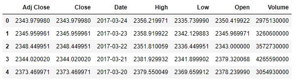
The dataset has a number of columns such as Open, Close etc. For the purposes of our exploration we will focus only on the Close price since we are interested in trends and not necessarily accuracy of returns.
In [3]:
df.head()
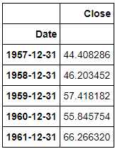
Take a look at the datatypes
In [4]:
df.info()
<class 'pandas.core.frame.DataFrame'>
Int64Index: 15429 entries, 0 to 118
Data columns (total 7 columns):
Adj Close    15429 non-null float64
Close        15429 non-null float64
Date         15429 non-null object
High         15429 non-null float64
Low          15429 non-null float64
Open         15429 non-null float64
Volume       15429 non-null int64
dtypes: float64(5), int64(1), object(1)
memory usage: 964.3+ KB
The datatype of the Date field needs to be converted into datetime64. This will help with plotting and computations as we shall see ahead.
In [5]:
df['Date'] = df.loc[:,'Date'].astype('datetime64[ns]')
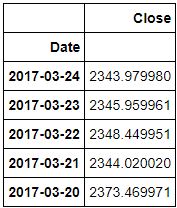
Extracting just the fields that we need into a new dataframe with daily data
In [6]:
dfd = df[["Date", "Close"]]
Setting the index of the dataframe to date
In [7]:
dfd = dfd.set_index('Date')
Take a look at the first few rows of the dataframe
In [8]:
dfd.head()
Sort the dataframe by date field
In [9]:
dfd = dfd.sort_index()
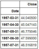
Create 2 new dataframes to hold the monthly average and yearly averages
In [10]:
dfm = dfd.resample('M').mean()
dfy = dfd.resample('Y').mean()
Take a look at the monthly average price. Notice that after sorting the initial rows go all the way back to 1957.
In [11]:
dfm.head()
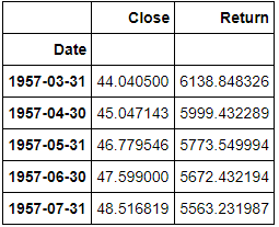
S&P 500 closed today Nov. 6, 2018 at 2747.62. What is the monthly return today had one unit been purchased monthly starting at the very first month that we have data for?
In [12]:
tday = 2747.62dfm['Return'] = (tday - dfm['Close'])/dfm['Close']*100
So if one had bought one unit of S&P 500 back in 1957 then it would at today’s price return 6138%.
In [13]:
dfm.head()
We calculated the returns for every day that we have data for in our dataframe dating back to 1957. Over the past 30 year period here is the return of a single unit of S&P 500 over time as of Nov. 6, 2018.
In [29]:
dfm.iloc[-360:,1].plot()

Now let us explore the yearly average data
In [15]:
dfy.head()
The chart above is useful to show the distribution of return over time. It confirms our intuition that returns are higher if stocks are held over a longer period and gradually decline as we hold them for lesser periods.
It will be interesting to see how much the five, ten, fifteen, twenty, twenty five and thirty year returns have changed over time. For this we will use the yearly average data.
In [16]:
dfy['5y'] = dfy['Close'].shift(5)
In [17]:
dfy['10y'] = dfy['Close'].shift(10)
dfy['15y'] = dfy['Close'].shift(15)
dfy['20y'] = dfy['Close'].shift(20)
dfy['25y'] = dfy['Close'].shift(25)
dfy['30y'] = dfy['Close'].shift(30)
Create a new dataframe to calculate the five year returns over time
In [18]:
fiveyearreturn = dfy[['Close','5y']].dropna()
fiveyearreturn['Return'] = (fiveyearreturn['Close'] - fiveyearreturn['5y'])/fiveyearreturn['5y']*100
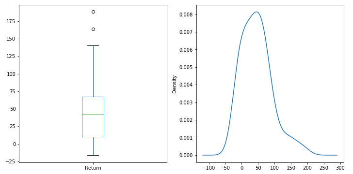
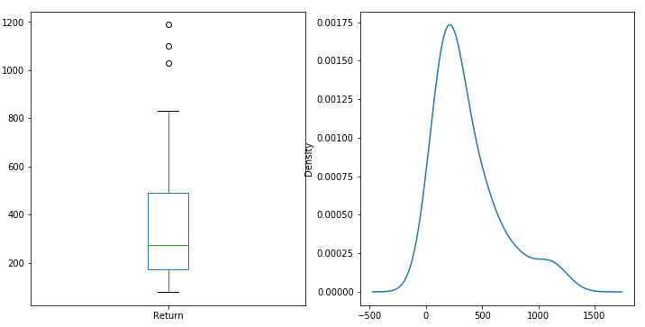
Create a boxplot and a kde plot of 5 year returns. The vast majority of the 5 year returns are above zero, which means that more often than not, it is hard to lose money in the market if held over a 5 year period. Although there are some years with negative returns. So had the index been purchased during some months, you could still be in the red after 5 years!
In [19]:
plt.figure(figsize=(12,6))
ax = plt.subplot(121)
fiveyearreturn['Return'].plot(kind='box')ax = plt.subplot(122)
fiveyearreturn['Return'].plot(kind='kde')
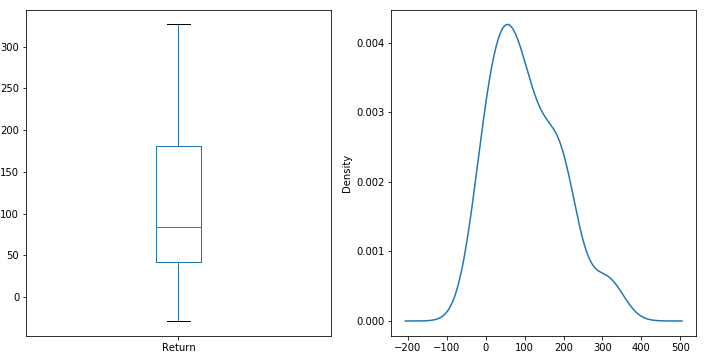
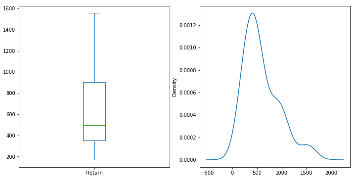
tenyearreturn = dfy[['Close','10y']].dropna()
tenyearreturn['Return'] = (tenyearreturn['Close'] - tenyearreturn['10y'])/tenyearreturn['10y']*100
A look at the 10 year returns shows that holding S&P 500 index over 10 years shows a largely positive returns, with a median return of 85%. Vast majority of the returns were over 100%. In some years the returns were above 300% while in others it may have been below 0%!
In [21]:
plt.figure(figsize=(12,6))
ax = plt.subplot(121)
tenyearreturn['Return'].plot(kind='box')
ax = plt.subplot(122)
tenyearreturn['Return'].plot(kind='kde')

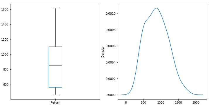
Repeating this exercise for 15, 20, 25 and 30 years will provide the following plots:
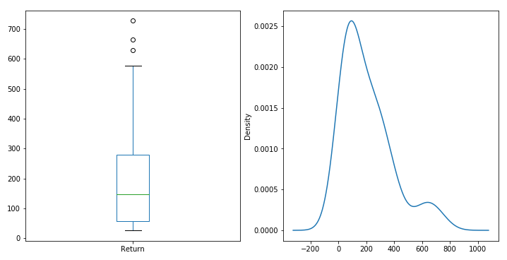
15 Years

20 Years

25 Years

30 Years
combinedreturn = pd.concat([fiveyearreturn['Return'], tenyearreturn['Return'],
          fifteenyearreturn['Return'], twentyyearreturn['Return'],
          x25yearreturn['Return'], thirtyyearreturn['Return']],axis=1, keys=['5y', '10y', '15y', '20y', '25y', '30y'])
Here is a side by side box plot of returns over 5, 10, 15, 20, 25 and 30 year periods.
In [28]:
combinedreturn.plot(kind='box', figsize=(8,6))
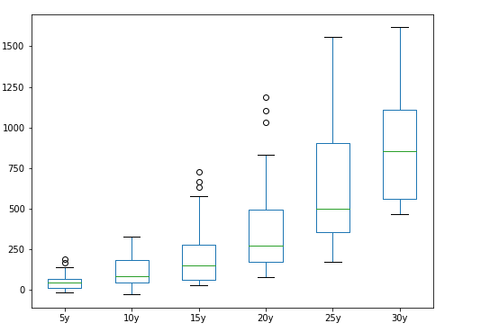
Combined Returns for 5,10,15,20,25 and 30 Year Returns
This chart aligns with our understanding of the markets that keeping money over longer term has a greater chance of producing returns and lesser chance of losing money, however some people may have had better success with some of their 20 year investments than those that they bought at the wrong time and held for longer than 20 years.
So what are those periods when the five year returns were negative? Some of these years are familiar such as 2003, 2009 etc.
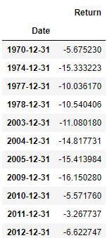
Years with Negative 5 year returns
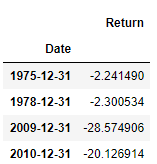
Years with Negative 10 year returns
The real question is if we were to buy the S&P 500 today, will we be under the water in 5 or 10 years?
Take 2010 and 10 years prior to 2010. What did S&P do during this period?
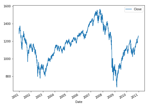
My son is 10 years from college. If I invest 10,000 in S&P today and 10 years from now when he is ready for college, and my S&P stock is worth 8000, then that could have a significant impact on our finances 10 years from now.
But the S&P need not look like this. Could it look like the 10 years leading up to 2000.
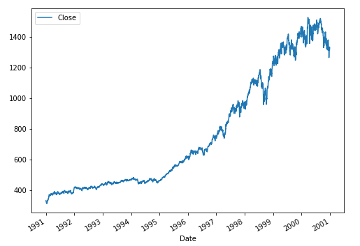
Now someone in 1991 would have done well in the market over a 10 year period.
Now let us look at the period from 2008 onward and compare it side by side with the period from 1991 through 2000. The returns have been spectacular in both periods, especially 2009 onward. The similarity is uncanny.
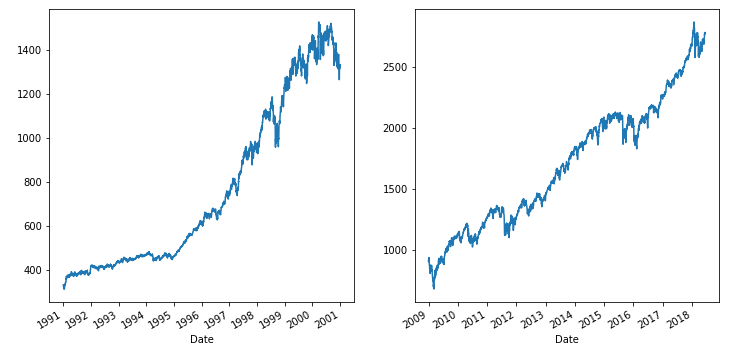
So it is quite possible that the S&P will look like the 2000 to 2010 period in the next 10 years which means there is a good chance that the stock market will yield a lower return 10 years from now.
